Notice that we built some very complicated images starting from very simple iterated function systems. For example, Barnsley's fern (as seen in class) requires just 4 affine transformations. This means that only 24 constants (6 constants per transformation) are enough to define this extraordinarily complex image. You can think of this as a compression of information - The information in that very complex image can be stored or represented by merely 24 numbers.
Our next goal is to somehow exploit this idea of compression of information by applying it to bitmap images in general. Bitmap images can take up quite a large amount of memory. Just a few images can take a big chunk out of our available disk space. If we could represent the information in an image with a few numbers we could just save those numbers instead of the original image. This would save a lot of memory for us. This is known as compression (the information is compressed to fit in a smaller file). Of course, most images are not in themselves fractals. Therefore, we'll have to modify our iterated function scheme to allow for less self-repetitive images. Even with a modified scheme for iterated function systems (called Partial Iterated Function Systems or PIFS), when we decompress the image (rebuild it from the stored constants), it will not look identical to the original images. Thus, we'll have to accept some loss of information in our images. Compression techniques that don't reproduce the exact original image are known as "lossy".
In a partial iterated function system, we begin by breaking the image area into non-overlapping subregions (called ranges). For simplicity, we'll assume that these subregions are squares all of equal sizes, although the text handed out in class gives several other more complicated (and more effective) ways to divide the image. Each of these ranges is assigned a square window on the image (called domains). For simplicity, we'll assume that these domains are squares of twice the width and height as the ranges, although there are many modifications you could make to that assumption. The domains may overlap, and may lie anywhere within the image. The idea is to begin with some random starting image, then to iterate as follows. For each range region, we calculate the new image by mapping the image in the corresponding domain region. The mapping is calculated for each of the ranges, and put together to create the first iteration. This process is repeated until the image "settles down" to a limiting image.
To map each domain to its corresponding range, we first solve the problem that the domain is twice the width and height of the range. We contract the image in the domain by a factor of 2 in each direction by averaging every 4-pixel square to get one pixel. Next, we transform the image into one of 8 possible orientations, namely, 4 possible rotations, or a mirror image with 4 possible rotations. (To simplify your program, you may omit this step. The sample files you'll be given have also eliminated this step.) Lastly, we scale the gray level to adjust the contrast and brightness. Thus, for each range region we must specify the location of the domain region, (optionally) which of the 8 orientations to use, a brightness level, and a contrast level.
The brightness and contrast level are designed to store information that will allow for differences in brightness and contrast from one part of the picture to another. The gray scale value of a mapped pixel is found by taking the gray scale g of the corresponding pixel in the domain, and calculating g*s + o, where s is the contrast constant and o is brightness constant for that particular region.
4 4 32 64
61 25 -0.270462 152.045
0 19 0.324733 93.5449
61 63 0.387698 90.7402
63 63 -0.400896 168.688
61 25 -0.296692 149.426
19 8 0.611102 42.5013
0 42 0.29549 118.214
51 21 0.476457 75.147
63 5 -0.360945 143.733
14 13 0.488712 32.2413
63 20 -0.554014 173.892
0 22 0.43626 99.8027
61 22 -0.557413 157.116
47 59 0.300475 45.5262
0 25 0.478591 85.8096
48 60 -0.479558 185.737
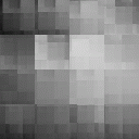
Here's the image generated by this file:

What has been described so far amounts to decompression of a PIFS file. Given a PIFS file, you know how to create an image from it. We have yet to describe how to compress an image. In other words, how do you get a list of PIFS transformations that will generate a given image, or an approximation of a given image?
To create a PIFS approximation of an image, you start by deciding how large you want your range rectangles to be. The smaller the rectangles, the more accurate your approximation will be, but smaller rectangles create larger PIFS files and take longer to calculate. The next step is to figure out, for each range rectangle, what part of the image most closely resembles it. To do this, you must traverse all possible domain rectangle possibilities and choose the best one. Remember that the domain rectangles are twice the size of the range rectangles and can lie anywhere within the image. For example, if your image is 256x256 pixels and your range rectangles are 8 pixels wide, then your domain rectangles are 16 pixels width, and there are 241 x 241 = 58081 possibilities. For each of these possibilities, you calculate the optimal constrast and brightness constants, along with a quantitative assessment of how good a match you have. Choose the best match, and write to a file its domain rectangle location, and the contrast and brightness constants. To calculate the optimal contrast and brightness constants and the evaluation of how good your match is, us the formulas given on page 21 of the text.
These calculations must be done for a large number of rectangles, and the calculations for each rectangle are involved. Therefore, this program is extremely computationally intensive. On reasonably-sized images, you should expect it to take a long time to complete execution. Run your program on a workstation that is not heavily used, and set the "nice" value to a nice value.
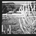
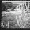
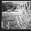
Here's some example images that show the loss associated with the compression. The first image is the original, and the second has been compressed and decompressed with a range region size of 8 pixels. The third has been compressed and decompressed with a range region of 4 pixels.
